Profile Viewer#
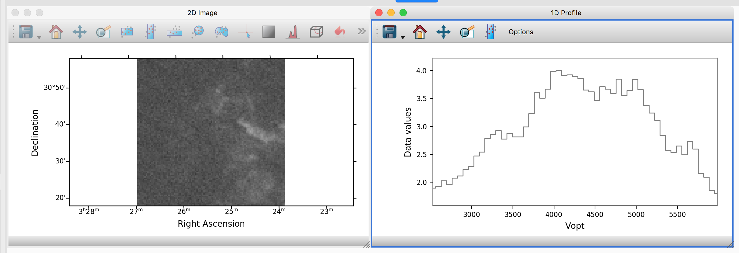
When using the image viewer on data with 3 or more dimensions, you have the option of extracting and analyzing 1D profiles (for Astronomers dealing with spectral cubes, this would be a spectrum). To compute a profile, click the profile button on an image viewer:

This will create a 1D profile viewer with the data collapsed along all but one axis (which you can select in the bottom left):

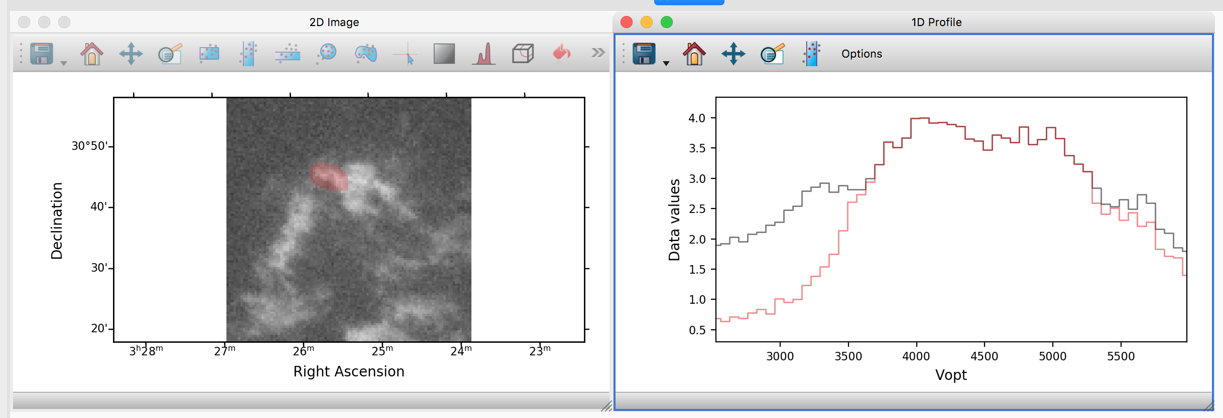
You can also create 1D profiles directly by dragging datasets onto the canvas rather than going via the image viewer. If the dataset has subsets, these will also result in profiles being computed in the profile viewer. If you don’t have any subsets yet, try and select a region in the image viewer, and you will then see the collapsed profile for that region in the profile viewer:

Interaction Modes#
The profile viewer has various advanced features that we now describe. To access these, click on the ‘Options’ button in the toolbar of the profile viewer.
Profile Fitting#
By clicking on the Fit tab, you can fit a model to the extracted spectrum. In this mode, you can click and drag on the spectrum to define a range over which to fit a mode. You can edit the range by dragging either of the edges. Clicking the fit button will add a best-fit model(s) to the plot (one model for each dataset and one for each subset). The dropdown lets you choose which model to fit to the data.
Different models have different settings, which you can adjust by clicking on the settings button. For example, the Gaussian fitter allows you to fix certain parameters, or limit them to specific ranges. For more information about customizing the models and/or fitting process, see Custom fitting plugins.
Cube Collapse#
The Collapse tab allows you to partially collapse the cube, and send the result back to the image viewer. As for fitting, you can draw and edit a range over which to collapse the data. Clicking ‘collapse’ will temporarily show a collapsed view of the data over the range in any image viewer currently showing the same data.
